Linear Regression and Gradient Descent

Some time ago, when I thought I didn’t have any on my plate (a gross miscalculation as it turns out) during my post-MSc graduation lull, I applied for a financial aid to take Andrew Ng’s Machine Learning course in Coursera. Having been a victim of the all too common case of very smart people being unable to explain themselves well and given Ng’s caliber, I didn’t think I would be able to wrap my head around the lectures. I’m on my 8th week now, and it’s honestly one of the things I look forward to when weekends roll around. However, my brain’s wiring dictates that my understanding of any concept only becomes granular when I force myself to write about it. Here is an attempt at linear regression and gradient descent.

Simple Linear Regression

In a simple linear regression problem, the relationship between two variables \(x\) and \(y\) (or \(h{_{\theta}}(x)\)) is governed by the line equation:

\[\begin{equation} h{_{\theta}}(x) = \theta_{0} + \theta_{1}x, \end{equation}\]

where \(\theta_{1}\) is the slope of the line, and \(\theta_{0}\) is the y-intercept.

It is used to predict values with a constant slope and within a continuous range. The idea is to fit this hypothesis to a training (existing) data so that it may be used to estimate \(y\) based on \(x\). Essentially, we need to look for the appropriate values for the parameters \(\theta_{0}\) and \(\theta_{1}\).

Cost Functions

What metric do we use to determine whether a combination of parameters is a good fit? Cost functions serve as a measure of how well or wrong the model is performing in terms of estimating the relationship between \(x\) and \(y\). Cost functions are typically expressed as the difference between the predicted value and the actual value. In the case of linear regression, the mean squared error (MSE) function is used:

\[\begin{equation} J(\theta _{_{0}}, \theta _{_{1}}) = \frac{1}{2m}\sum_{i=1}^{m}(h_{\theta }(x^{(i)}) - y^{(i)})^{2} \end{equation}\]

Our ultimate goal is to minimize the cost function. In other words, we want to minimize the difference between the predicted and actual values (minimize \(J(\theta _{_{0}}, \theta _{_{1}})\)).

Gradient Descent

Keeping in mind that our ultimate goal is to minimize the cost function \(J(\theta _{_{0}}, \theta _{_{1}})\), we can start with some random values for \(\theta_{0}\) and \(\theta_{1}\), and keep changing or updating the values until we end up at a minimum. To implement this, we can use gradient descent, an efficient optimization algorithm that allows a model to learn the gradient or direction it should take to reduce errors. The algorithm can be formally presented as follows:

\[\begin{equation} \text{ repeat until convergence: \{}\\ \theta_0{} := \theta_0{} - \alpha\frac{1}{m}\sum_{i=1}^{m}(h_\theta(x^{(i)}) - y^{(i)})\\ \theta_1{} := \theta_1{} - \alpha\frac{1}{m}\sum_{i=1}^{m}((h_\theta(x^{(i)}) - y^{(i)})\cdot x^{(i)})\\ \text{\}} \end{equation}\]

where \(\alpha\) is the learning rate or how quickly we approach the minimum.

We know we have succeeded when the cost function is at its minimum. Graphically, if we put \(\theta_0\) on the x-axis, \(\theta_1\) on the y-axis, and the cost function \(J(\theta _{_{0}}, \theta _{_{1}})\) on the vertical z-axis, this looks like reaching the bottom areas of this graph:

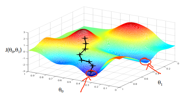
Visualization of gradient descent. Credit: Andrew Ng (Machine Learning).

Linear Regression with Multiple Variables

For multivariate linear regression, wherein multiple correlated dependent variables are being predicted, the gradient descent equation maintains the same form and is repeated for the \(n\) features being taken into consideration:

\[\begin{equation} \text{ repeat until convergence: \{}\\ \theta_j{} := \theta_j{} - \alpha\frac{1}{m}\sum_{i=1}^{m}(h_\theta(x^{(i)}) - y^{(i)})\cdot x_{j}^{(i)}\\ \text{ for j:= 0...n}\\ \text{\}} \end{equation}\]

Learning Rate

Caution must be exercised when choosing the learning rate \(\alpha\). A sufficiently small \(\alpha\) will cause the cost function \(J(\theta)\) to decrease on every iteration. However, if \(\alpha\) is too small, the gradient descent will take a while to converge. If \(\alpha\) is too large, \(J(\theta)\) may not decrease on every iteration and may fail to converge.

Speeding Up Gradient Descent

The process of converging to a minimum can be sped up through two techniques, namely feature scaling and mean normalization. Feature scaling refers to the process of framing the features within the \(-1 < x < 1\) range, and it involves dividing the input values by the range of the input variable (i.e., maximum value minus the minimum value). Mean normalization, on the other hand, necessitates the subtraction of an average value from the values, in order to make the features have an approximately zero mean. To implement feature scaling and mean normalization, the input values can be adjusted as follows:

\[\begin{equation} x_{i:=}\frac{x_{i} - \mu_{i}}{s_{i}}, \end{equation}\]

where \(\mu_{i}\) is the average of all the values for feature \((i)\), and \(s_{i}\) may be the range of the input variable (i.e., maximum value minus the minimum value) or the standard deviation.

Implementation of Linear Regression in R

For a sample implementation of linear regression in R, let’s use the built-in cars dataset.

> data("cars") ## Load the cars dataset
> head(cars) ## Inspect the first few lines of the dataset
  speed dist
1     4    2
2     4   10
3     7    4
4     7   22
5     8   16
6     9   10

To visually inspect whether there is a linear relationship between the variables in the dataset, draw a scatter plot:

scatter.smooth(x=cars$speed, y=cars$dist, main="Dist ~ Speed") ## Create scatter plot

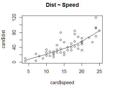
Scatter plot of the "cars" dataset.

The scatter plot and the smoothing line suggest a linear relationship between the variables dist and speed.

We can also check the level of linear dependence between dist and speed by calculating their correlation:

> cor(cars$speed, cars$dist) ## Calculate correlation
[1] 0.8068949

A high positive correlation of 0.8068949 suggests that dist increases along with speed. We can now build a linear model using the lm function:

> linearReg <- lm(dist ~ speed, data=cars) ## Perform linear regression
> linearReg$coefficients ## Get the values of the parameters
(Intercept)       speed 
 -17.579095    3.932409 

Therefore, we can model the cars dataset using the formula:

\[\begin{equation} dist=-17.579095+3.932409\cdot speed \end{equation}\]