Making Maps with ggplot2

I remember looking at Freedom House’s beautiful (but alarming) set of visualizations on the status of global democracy in 2018 with a burning curiosity about the code underlying the colored maps. Given the biological nature of the data that I regularly work with, I already abandoned all hope of making such fancy maps out of genuine necessity—not until the unveiling of the dataviz challenge of David McCandless of Information is Beautiful and the World Government Summit. I have no intention of participating, but I love me some tidy data that I can cop without scraping. Now on to the code:

Objective

• To use ggplot2 to plot the global human development index (HDI). The HDI metric from the United Nations Development Program (UNDP) is a summary measure of the average achievement of a country in key dimensions of human development: a long and healthy life, being knowledgeable, and a decent standard of living (value ranges from 0 to 1, higher = better).

Load the libraries

library(dplyr)
library(stringr)
library(ggplot2)
library(maps)

options(scipen = 999) ## To disable scientific notation

The maps package contains outlines of several continents, countries, and states (examples: world, usa, state) that have been with R for a long time. maps has its own plotting function, but we will use the map_data() function of ggplot2 to make a data frame that ggplot2 can operate on.

Making a data frame from map outlines

world <- map_data("world")
head(world)

##        long      lat group order region subregion
## 1 -69.89912 12.45200     1     1  Aruba      <NA>
## 2 -69.89571 12.42300     1     2  Aruba      <NA>
## 3 -69.94219 12.43853     1     3  Aruba      <NA>
## 4 -70.00415 12.50049     1     4  Aruba      <NA>
## 5 -70.06612 12.54697     1     5  Aruba      <NA>
## 6 -70.05088 12.59707     1     6  Aruba      <NA>

The new world data frame has the following variables: long for longitude, lat for latitude, group tells which adjacent points to connect, order refers to the sequence by which the points should be connected, and region and subregion annotate the area surrounded by a set of points.

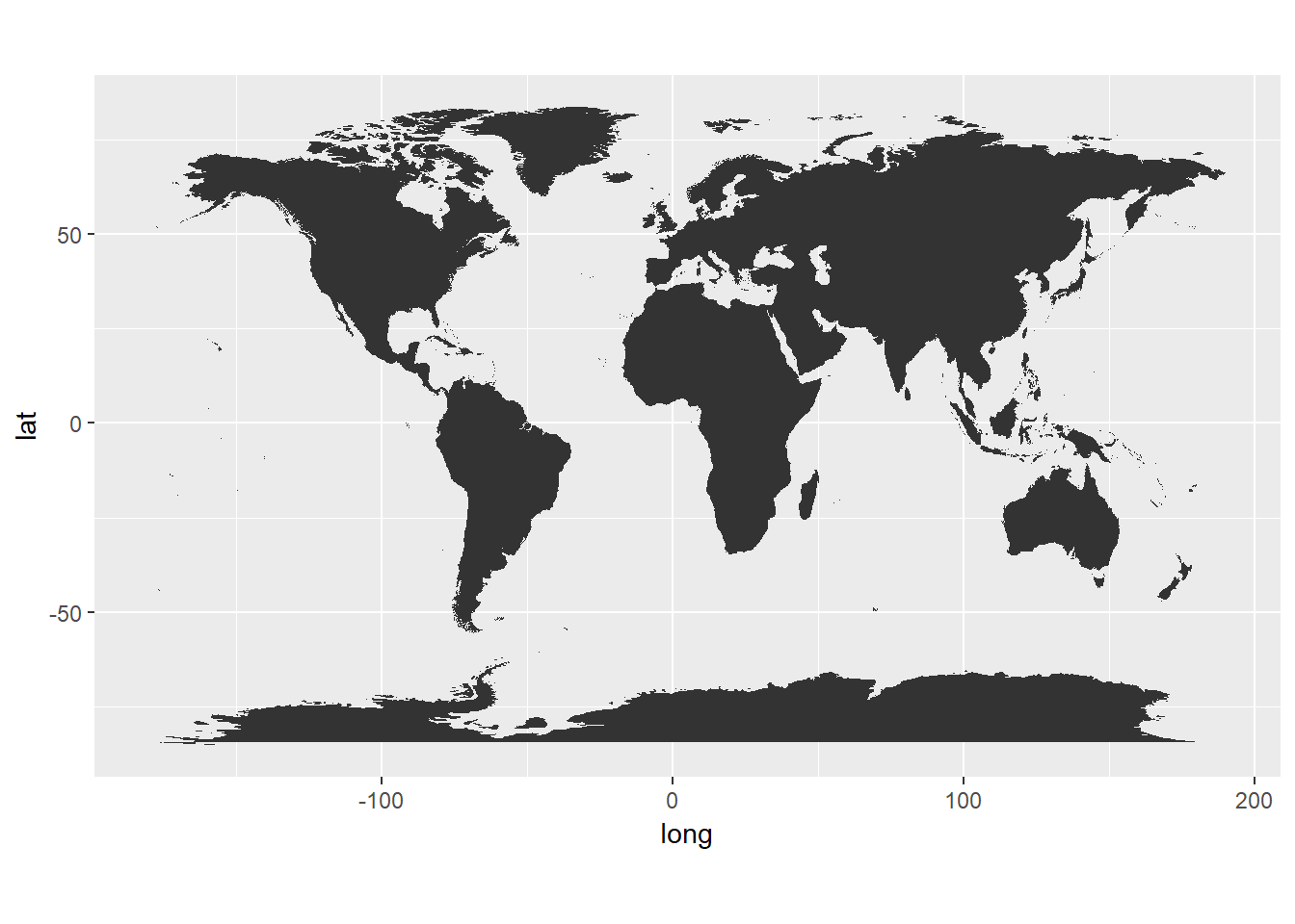
Making a simple world map

geom_polygon() draws maps with gray fill by default and coord_fixed() specifies the aspect ratio of the plot (every y unit is 1.3 times longer than the x unit).

world <- map_data("world")
worldplot <- ggplot() +
  geom_polygon(data = world, aes(x=long, y = lat, group = group)) + 
  coord_fixed(1.3)
worldplot

Loading and cleaning the data

Let’s load the data from the World Data Visualization Prize challenge. For the sake of clarity, we select only the indicator, human.development.index, and ISO.Country.code columns. Within the select() function, the indicator column is renamed to region for the inner_join() we will do later between the world and worldgovt datasets.

worldgovt <- read.csv("./world-govt.csv", header = TRUE)
worldgovt <- select(worldgovt, region = indicator, "HDI" = `human.development.index`, "CC" = ISO.Country.code)
head(worldgovt)

##              region   HDI  CC
## 1       Afghanistan 0.498 AFG
## 2           Albania 0.785 ALB
## 3           Algeria 0.754 DZA
## 4           Andorra 0.858 AND
## 5            Angola 0.581 AGO
## 6 Antigua & Barbuda 0.780 ATG

There will definitely be disagreements between the nomenclature of world$region and worldgovt$region, and we will fix them with this code snippet :

## Check for disagreements between the two datasets
diff <- setdiff(world$region, worldgovt$region)

## Clean the dataset accordingly
worldgovt <- worldgovt %>%
  ## Recode certain entries
  mutate(region = recode(str_trim(region), "United States" = "USA",
                            "United Kingdom" = "UK",
                            "Korea (Rep.)" = "South Korea",
                            "Congo (Dem. Rep.)" = "Democratic Republic of the Congo",
                            "Congo (Rep.)" = "Republic of Congo")) %>%
  ## Editing the "North Korea" entry is a little trickier for some reason
  mutate(region = case_when((CC == "PRK") ~ "North Korea",
                               TRUE ~ as.character(.$region)))

## Make the HDI numeric
worldgovt$HDI <- as.numeric(as.character(worldgovt$HDI))

Merge the datasets

Before we draw the map with ggplot2, let’s merge the two datasets by region:

worldSubset <- inner_join(world, worldgovt, by = "region")
head(worldSubset)

##       long      lat group order      region subregion   HDI  CC
## 1 74.89131 37.23164     2    12 Afghanistan      <NA> 0.498 AFG
## 2 74.84023 37.22505     2    13 Afghanistan      <NA> 0.498 AFG
## 3 74.76738 37.24917     2    14 Afghanistan      <NA> 0.498 AFG
## 4 74.73896 37.28564     2    15 Afghanistan      <NA> 0.498 AFG
## 5 74.72666 37.29072     2    16 Afghanistan      <NA> 0.498 AFG
## 6 74.66895 37.26670     2    17 Afghanistan      <NA> 0.498 AFG

Plot the final map

For brevity, I combined all of the elements I want to be absent in the final plot in plain. To color each country or region with its corresponding HDI value, I mapped the fill aesthetic to HDI using the RdBu palette from RColorBrewer.

## Let's ditch many of the unnecessary elements
plain <- theme(
  axis.text = element_blank(),
  axis.line = element_blank(),
  axis.ticks = element_blank(),
  panel.border = element_blank(),
  panel.grid = element_blank(),
  axis.title = element_blank(),
  panel.background = element_rect(fill = "white"),
  plot.title = element_text(hjust = 0.5)
)

worldHDI <- ggplot(data = worldSubset, mapping = aes(x = long, y = lat, group = group)) + 
  coord_fixed(1.3) +
  geom_polygon(aes(fill = HDI)) +
  scale_fill_distiller(palette ="RdBu", direction = -1) + # or direction=1
  ggtitle("Global Human Development Index (HDI)") +
  plain

worldHDI

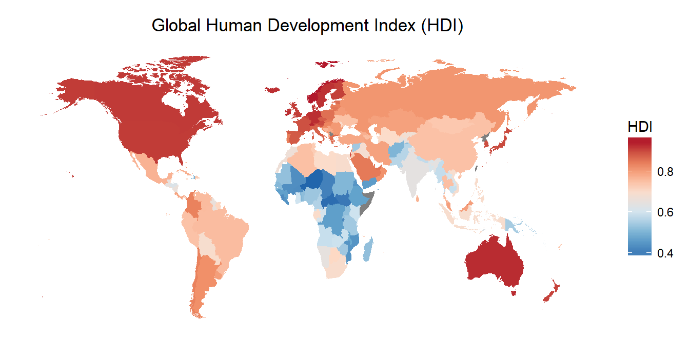
What can we say about the data?

At a glance, majority of African countries have low HDI while the superpowers have high HDI. In the interest of comparing government policy priorities, what would be interesting to look at later on are countries with the same Gross National Income (GNI) per capita but with different human development outcomes.